Examples
Plotting Experiments onto Multiple Axes
In order to allow for generated more complicated figures, the plotExpt function supports passing an instance matplotlib.pyplot.Axes object.
import DAPyr as dap
import matplotlib.pyplot as plt
expt = dap.Expt('Plotting_example', {'expt_flag': 0, 'model_flag': 0, 'T': 200, 'seed': 1})
dap.runDA(expt)

plt.close()
#Create a Figure and Axes instance, make sure to specify a 3d projection
fig, axes = plt.subplots(1, 2, subplot_kw = {'projection': '3d'})
T1, T2 = 10, 150
dap.plotExpt(expt, T = T1, ax = axes[0])
dap.plotExpt(expt, T = T2, ax = axes[1])
axes[0].set_title('Experiment at time T = {}'.format(T1))
axes[1].set_title('Experiment at time T = {}'.format(T2))

#You many then modify the Axes instance to adjust for axes limits
new_xlim = (-9.5, -7.0)
new_ylim = (-9.5, -6.0)
new_zlim = (24, 30)
for ax in axes:
      ax.set_xlim(new_xlim)
      ax.set_ylim(new_ylim)
      ax.set_zlim(new_zlim)
plt.show()
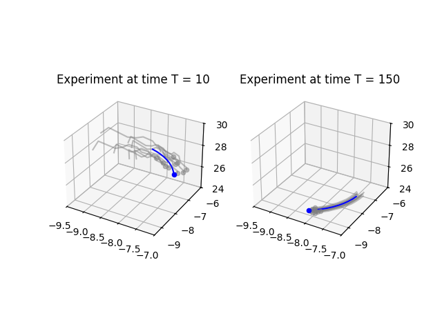
A figure with multiple plotExpt instances at different time steps in the experiment.
Ensuring Same Starting State between Experiments
When setting up experiments, you may want to ensure that two experiments with different parameter configuration have the same states. As in, the same model truth (\(x_t\)), observations (\(Y\)), and initial ensemble state (\(x_f^0\)).
Using the seed parameter
The seed parameter in the Expt class sets the seed of the random number generator used to spin up the initial ensemble state, \(x_f^0\).
import DAPyr as dap
import numpy as np
expt1 = dap.Expt('enkf_run', {'expt_flag': 0, 'Ne': 15, 'seed': 10})
expt2 = dap.Expt('lpf_run', {'expt_flag': 1, 'Ne': 15, 'seed': 10})
np.allclose(expt1.getParam('xf_0'), expt2.getParam('xf_0'))
True
Note
Setting the seed parameter will only ensure equal ensemble initial states if ensemble sizes are equal between experiments. Additionally, the seed parameter does not enforce equality for either model truth or observation state vectors.
Using the copyStates method
The copyStates method ensures all three state vectors are copied from another experiment. However, one must be careful when copying states to another experiment with different modified parameters, as many parameters directly influence the state vectors. Major differences between experiment will be caught and raise exceptions. For example, attempting to copy the state vectors from an experiment where h_flag = 0 to an experiment with h_flag = 1 will throw an exception. On the contrary, copying the state vectors from an experiment where l05_I = 1 to an experiment where l05_I = 12 will result in incorrect model integration.
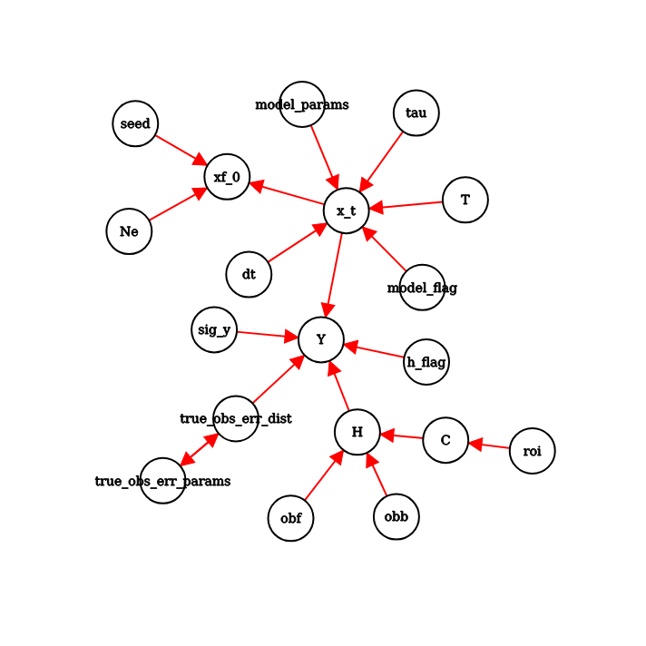
State vector dependency based on parameter. Edges point to what parameters influence what state vectors during spin-up.
import DAPyr as dap
import numpy as np
expt1 = dap.Expt('enkf_run', {'expt_flag': 0, 'Ne': 15})
expt2 = dap.Expt('lpf_run', {'expt_flag': 1, 'Ne': 15})
np.allclose(expt1.getParam('xf_0'), expt2.getParam('xf_0'))
False
#Copy states of expt1 onto expt2
expt2.copyStates(expt1)
np.allclose(expt1.getParam('xf_0'), expt2.getParam('xf_0'))
True
np.allclose(expt1.getParam('xt'), expt2.getParam('xt'))
True
np.allclose(expt1.getParam('Y'), expt2.getParam('Y'))
True
Directly modifying the Expt.states attribute
For more complex modifications and edit you can directly access the state vectors through the Expt.states attribute. The states attribute is a dictionary containing the model truth (xt), observations (Y), and initial ensemble state (xf_0).
import DAPyr as dap
import numpy as np
expt = dap.Expt('enkf_run', {'expt_flag': 0, 'Ne': 15})

#Add additional noise to initial ensemble state vector
Nx, Ne = expt.states['xf_0'].shape
expt.states['xf_0'] = expt.states['xf_0'] + np.random.randn(Nx, Ne)
Specifying Alternate Observation Error Distributions
During spin-up, observations can be sampled from a user-prescribed distribution. This is accomplished by configuring the true_obs_err_dist and true_obs_err_params parameters when initializing an experiment. Currently supported distributions can be found here.
import DAPyr as dap
import matplotlib.pyplot as plt

# Corresponds to state-dependent Gaussian observation error.

SD_GAUSSIAN_ERR = 1

# Errors have mean -2 and variance 1 when the state is negative,
# and mean 3 and variance 0.25 when the state is positive.

SD_GAUSSIAN_PARAMS = {'mu1': -2.0, 'sigma1': 1, 'mu2': 3.0, 'sigma2':.5, 'threshold': 0}

e_sd_gauss = dap.Expt('Using Different Obs Errors in DAPyr', {'expt_flag': 1,
                        'model_flag':1,
                        'localize':1,
                        'obf': 1,
                        'seed': 1,
                        'true_obs_err_dist': SD_GAUSSIAN_ERR,
                        'true_obs_err_params': SD_GAUSSIAN_PARAMS,
                        'Ne':80,
                        'T': 500})


xf_0, xt, y = e_sd_gauss.getStates()

y = y.flatten()
xt = xt.flatten()

plt.hist(y-xt, bins=50)
plt.show()
We can confirm that observation errors were sampled from the prescribed distribution:

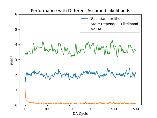
When using a data assimilation method that can accommodate non-Gaussian observation errors, we can choose an alternate form of the likelihood of observations given model states by setting assumed_obs_err_dist and assumed_obs_err_params. This is also how we can set a different variance for a Gaussian observation error. Below, we run data assimilation experiments with the above observation errors with Gaussian likelihoods and with likelihoods that correspond to the true observation error distribution.
e_sd_gauss_l = dap.Expt('Assuming a Different Form of the Likelihood', {'expt_flag': 1,
                        'model_flag':1,
                        'localize':1,
                        'obf': 1,
                        'seed': 1,
                        'true_obs_err_dist': SD_GAUSSIAN_ERR,
                        'true_obs_err_params': SD_GAUSSIAN_PARAMS,
                        'assumed_obs_err_dist': SD_GAUSSIAN_ERR,
                        'assumed_obs_err_params': SD_GAUSSIAN_PARAMS,
                        'Ne':80,
                        'T': 500})

# for comparison
e_noda = dap.Expt('Assuming a Different Form of the Likelihood', {'expt_flag': 2,
                        'model_flag':1,
                        'localize':1,
                        'obf': 1,
                        'seed': 1,
                        'Ne':80,
                        'T': 500})

dap.runDA(e_sd_gauss)
dap.runDA(e_sd_gauss_l)
dap.runDA(e_noda)

plt.plot(e_sd_gauss.rmse, label='Gaussian Likelihood')
plt.plot(e_sd_gauss_l.rmse, label='State-Dependent Likelihood')
plt.plot(e_noda.rmse, label='No DA')
plt.legend()
plt.ylim((0,6))
plt.xlabel('DA Cycle')
plt.ylabel('RMSE')
plt.title('Performance with Different Assumed Likelihoods')
plt.show()